Logistic regression from scratch

Outlining the problem

We have $n$ observations of $d$ dimensional data $\boldsymbol{x} = (x_1, x_2, ... x_d)$. For each observation $\boldsymbol{x^i}$ we have a corresponding label $y^i \in \{0, 1\}$. Now, we want to build a model that can predict a label given some unseen observation $\boldsymbol{x^k}$. Essentially we want to find a function that can model the following probability accurately

$P(Y=y | X = \boldsymbol{x^k})$

Since we only have two classes to predict we can keep our model simple with a single output

$P(Y=1 | X = \boldsymbol{x^k}) = p^k$

$P(Y=0 | X = \boldsymbol{x^k}) = 1-p^k$

To build our model let’s start with something simple like linear regression and multiply our observations with a set of learned weights $\boldsymbol{w}$ and add a bias $\beta$ to get our probabilities. Predicting the probability $p^k$ for an observation $\boldsymbol{x^k}$ is then equal to

$P( Y = 1 | X = \boldsymbol{x^k}) = \boldsymbol{w^T}\boldsymbol{x^k} + \beta = w_1 x^k_1 + w_2 x^k_2 + ... w_d x^k_d + \beta = p^k$

Let’s add an extra weight $w_{d+1}$ and $x_{d+1} = 1$ to all our observations to remove the extra bias term and simplify our expression

$P( Y = 1 | X = \boldsymbol{x^k}) = \boldsymbol{w^T}\boldsymbol{x^k}$

So now we have a linear regression model. But notice how this does not work for classification since the model will output any real number instead of a probability. Our probabilities need to take on values between $0$ and $1$ so we need to somehow squash the output of our model.

Forcing our model to output probabilities

Now there’s several functions we can use to achieve this. Let’s start with looking at a function called the logistic function:

$f(x) = \frac{1}{1+e^{-x}}$

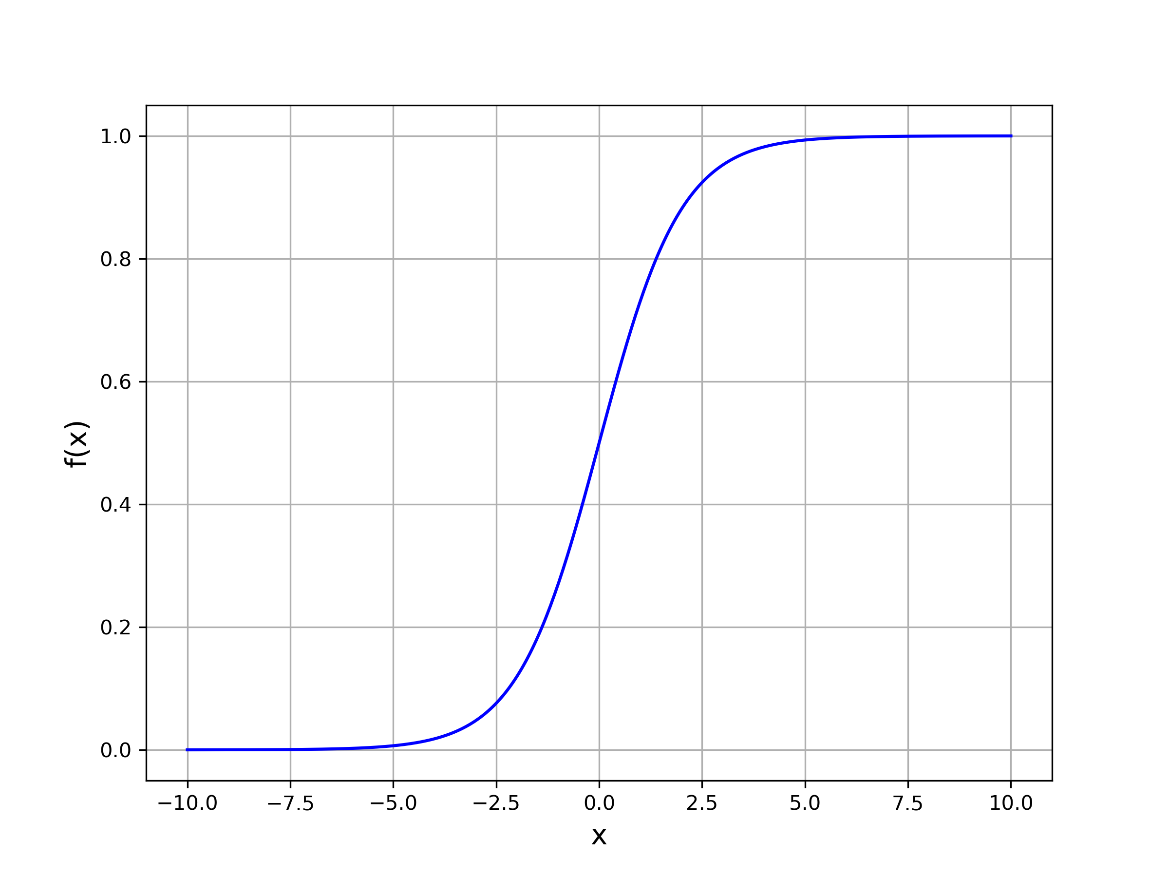
Notice how the function squashes our model’s output between $0$ and $1$. Let’s plug in our linear transformation into this model and voila! Our model can now output a probability given an observation $\boldsymbol{x}$.

$P( Y=1 | X = \boldsymbol{x}) = \frac{1}{1+e^{-\boldsymbol{w^T}\boldsymbol{x}}}$

The intuition behind the logistic function

But why use the logistic function instead of some other squashing function? It turns out the logistic function allows us to interpret the output of the linear transformation, $\boldsymbol{w^T}\boldsymbol{x}$ quite nicely. Starting with our model’s definition let’s solve for our linear transformation:

$\frac{1}{1+e^{-\boldsymbol{w^T}\boldsymbol{x}}} = p$

Multiplying with our denominator on both sides of the equation

$1 = (1 + e^{-\boldsymbol{w^T}\boldsymbol{x}}) p$

Expanding the right side

$1 = p + e^{-\boldsymbol{w^T}\boldsymbol{x}} p$

Subtract $p$ from both sides and then dividing both sides with $p$

$\frac{1 - p}{p} = e^{-\boldsymbol{w^T}\boldsymbol{x}}$

Take the natural logarithm

$\ln \left( \frac{1 - p}{p} \right) = -\boldsymbol{w^T}\boldsymbol{x}$

Multiply by $-1$ to isolate our linear transformation

$-\ln \left( \frac{1 - p}{p} \right) = \boldsymbol{w^T}\boldsymbol{x}$

Our linear transformation can therefore be expressed as

$\boldsymbol{w^T}\boldsymbol{x} = \ln \left( \frac{p}{1 - p} \right)$

The fraction $\frac{p}{1 - p}$ is not a coincidence, it denotes the odds of an event given probability $p$. For example if the probability of an event is 80%, we can calculate the odds being 4:1.¹ We can see that our model is trying to find a linear relationship between the log-odds and our input data $\boldsymbol{x}$. This is a key assumption of logistic regression, and this will help us interpret our weights just like in linear regression. For example, we can easily see how increasing a weight $w_d$ will correspond to a $x_d$ change in log-odds. Similarly, our bias term $\beta$ represents the log-odds of our model if our input vector $\boldsymbol{x}$ is 0.

Finding our loss function

Now, we have our formula for making predictions, but how do we train our model so we can find the optimal weights $\boldsymbol{w}$?

Basically we want to find $\boldsymbol{w}$ such that $P(Y | X)$, known as the likelihood, is maximized. This process is known as maximum likelihood estimation.²

$\argmax_w \mathcal{L}(\boldsymbol{w}) = \argmax_w P(Y | X)$

Assuming our observations are independent this becomes:

$\argmax_w \mathcal{L}(\boldsymbol{w}) = \argmax_w \prod_{i=1}^{n} P(y^i | \boldsymbol{x^i})$

Now products can be a bit of a hazzle to work with, they can be messy to differentiate and often run into numerical stability issues if we multiply a lot of small numbers. We can apply the natural logarithm here since it’s a monotonically increasing function and therefore doesn’t affect our choice of $\boldsymbol{w}$. Using the product rule this simply becomes a sum.

$\argmax_w \mathcal{L}(\boldsymbol{w}) = \argmax_w \sum_{i=1}^{n} \ln{P(y^i | \boldsymbol{x^i})}$

This formula is referred to as the log-likelihood. Conventionally, we minimize the negative likelihood which is equivalent to maximizing the log likelihood (NLL).

$NLL = \argmin_w - \mathcal{L}(\boldsymbol{w} | X) = \argmin_w - \sum_{i=1}^{n} \ln{P(y^i | \boldsymbol{x^i})}$

We can interpret $P(y^i | \boldsymbol{x^i})$ as a Bernoulli trial with probability of success being $p$, that is

$P(Y=y | X = \boldsymbol{x}) \sim Bernoulli(p)$

Where the probability mass function for a Bernoulli trial is

$P(Y=y | X = \boldsymbol{x}) = {p}^{y} (1-p)^{1-y}$

Now, let’s enter our logistic model into the PMF

$P(Y = y | X = \boldsymbol{x}) = \left( \frac{1}{1+e^{-\boldsymbol{w^T}\boldsymbol{x}}} \right)^y \left( 1-\frac{1}{1+e^{-\boldsymbol{w^T}\boldsymbol{x}}}\right)^{1-y}$

Finally, plugging this into the negative log likelihood formula above

$NLL = \argmin_w - \sum_{i=1}^{n} \left[ \ln \left( \left( \frac{1}{1+e^{-\boldsymbol{w^T}\boldsymbol{x^i}}} \right)^{y^i} \left( 1-\frac{1}{1+e^{-\boldsymbol{w^T}\boldsymbol{x^i}}} \right)^{1-y^i} \right)\right]$

Using the product rule for logarithm we can simplify this to

$NLL = \argmin_w - \sum_{i=1}^{n} \left[ y^i \ln \left( \frac{1}{1+e^{-\boldsymbol{w^T}\boldsymbol{x^i}}} \right) + (1-y^i) \ln \left( 1 - \frac{1}{1+e^{-\boldsymbol{w^T}\boldsymbol{x^i}}} \right) \right]$

Finding the $w$ that minimizes the negative log-likelihood.

Our likelihood function does not have a closed form solution like linear regression. So we need to use a numerical optimization algorithm to find our optimal $\boldsymbol{w}$. A common choice is gradient descent, first we find the derivative of the function we are trying to optimize. Then take fixed size steps down the gradient until we arrive at the minima or in other words the optimal choice of $w$ that minimizes the negative log likelihood.

We’ll make one small change to our negative log likelihood. We’ll take the average of the likelihoods across our observations so that our dataset size doesn’t increase our log likelihood score. Our cost function is therefore defined as follows

$J(w) = - \frac{1}{n} \sum_{i=1}^{n} y^i \left[ \ln \left( \frac{1}{1+e^{-\boldsymbol{w^T}\boldsymbol{x^i}}} \right) + (1-y^i) \ln \left( 1 - \frac{1}{1+e^{-\boldsymbol{w^T}\boldsymbol{x^i}}} \right) \right]$

Let’s simplify a bit further by using the rule for logarithms of fractions

$J(w) = - \frac{1}{n} \sum_{i=1}^{n} \left[ -y^i \ln ({1+e^{-\boldsymbol{w^T}\boldsymbol{x^i}}}) + (1-y^i)(-\boldsymbol{w^T}\boldsymbol{x^i} - \ln(1+e^{-\boldsymbol{w^T}\boldsymbol{x^i}})) \right]$

And simplifying further

$J(w) = - \frac{1}{n} \sum_{i=1}^{n} \left[ y^i \boldsymbol{w^T}\boldsymbol{x^i} -\boldsymbol{w^T}\boldsymbol{x^i} - \ln(1+e^{-\boldsymbol{w^T}\boldsymbol{x^i}}) \right]$

Now the gradient of the cost function w.r.t. $w$ is simply

$\nabla J(W) = - \frac{1}{n}\sum_{i=1}^{n} \left( y^i \boldsymbol{x^i} - \boldsymbol{x^i} + \frac{e^{-\boldsymbol{w^T}\boldsymbol{x^i}}\boldsymbol{x^i}}{1+e^{-\boldsymbol{w^T}\boldsymbol{x^i}}} \right)$

Simplifying a bit we end up with:

$\nabla J(W) = \frac{1}{n}\sum_{i=1}^{n} \left( \frac{1}{1+e^{-\boldsymbol{w^T}\boldsymbol{x^i}}} - y^i \right) \boldsymbol{x^i}$

And we recognize that fraction. It’s simply the logistic function! We now have all the tools we need to put this knowledge to practice!

Tying it all together in Python

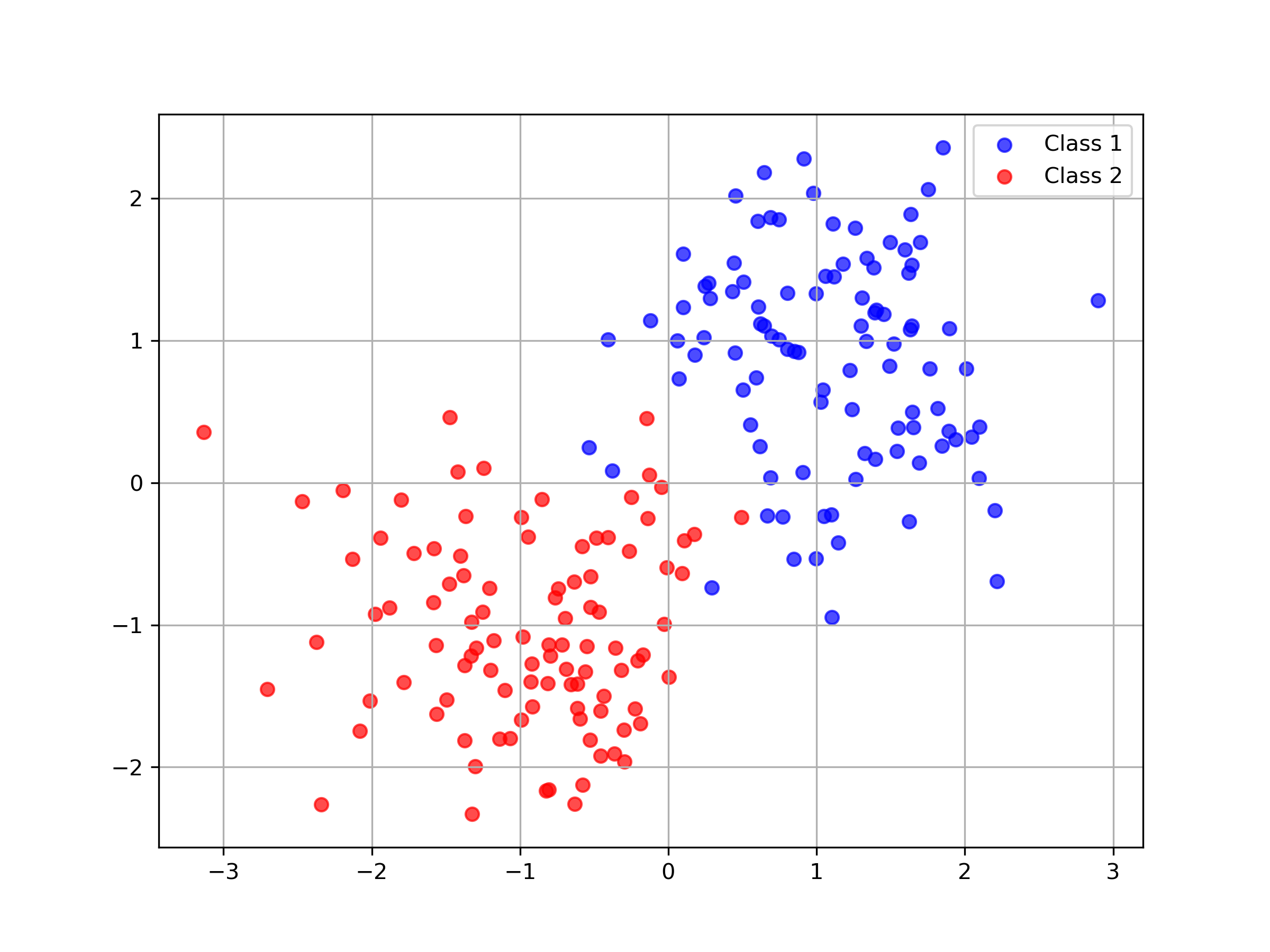
Let’s generate some very simple dataset with two classes that are linearly separable.

# Make this reproducible 
np.random.seed(1337)

# Define means and covariances for two classes
class_1_mean = [1, 1]
class_1_cov = [[0.25, 0], [0, 0.25]]

class_2_mean = [-1, -1]
class_2_cov = [[0.25, 0], [0, 0.25]]

# Generate n samples from the multivariate normal distribution for both classes
x1 = np.random.multivariate_normal(class_1_mean, class_1_cov, n)
x2 = np.random.multivariate_normal(class_2_mean, class_2_cov, n)

y1 = np.ones(n)    
y2 = np.zeros(n)  

x = np.vstack((x1, x2))
y = np.hstack((y1, y2))

Plotting this data we get a nice figure. We can see that the data is basically linearly separable, our model should perform quite well here.

Now let’s set up our logistic regression model and how we train it so that the weights of our model are optimized. Note that there’s a whole wizardry field on how to optimize hyperparameters like the step size. For the purposes of this post we’ll just pick something reasonable.

def predict(x, w):
    prob = sigmoid(x, w)
    return (prob >= 0.5).astype(int)

def sigmoid(x, w): 
    return 1 / (1 + np.exp(-np.dot(x, w)))

def loss(x, y, w):
    prob = sigmoid(x, w)
    loss = -1/x.shape[0] * np.sum(y * np.log(prob) + (1-y)*np.log(1-prob))
    return loss

def accuracy(y, y_pred):
    return np.mean(y == y_pred)

def gradient(x,y,w):
    n = x.shape[0]
    return (1/n) * x.T @ (sigmoid(x,w)-y)

# Set up our hyper parameters
training_iters = 200
learning_rate = 0.05

# For reproducibility
np.random.seed(1337) 

# Add a column of ones for our bias
x = np.hstack((x,np.ones((x.shape[0], 1))))

# Define our weight array, two for our dimensions and 1 for bias
w = np.random.normal(size=3)

# Let's train!      
for i in range(training_iters):
    w -= learning_rate*gradient(x,y,w)
    if i % 10 == 0:
        print("NLL is {}".format(loss(x,y,w)))

# Now that we have the model let's get out predictions
y_pred = predict(x, w)
print("Accuracy is {}".format(accuracy(y, y_pred)))              

We can plot the decision boundary of our model: where $P(Y=y | X) = 0.5$ at various points during the training process.

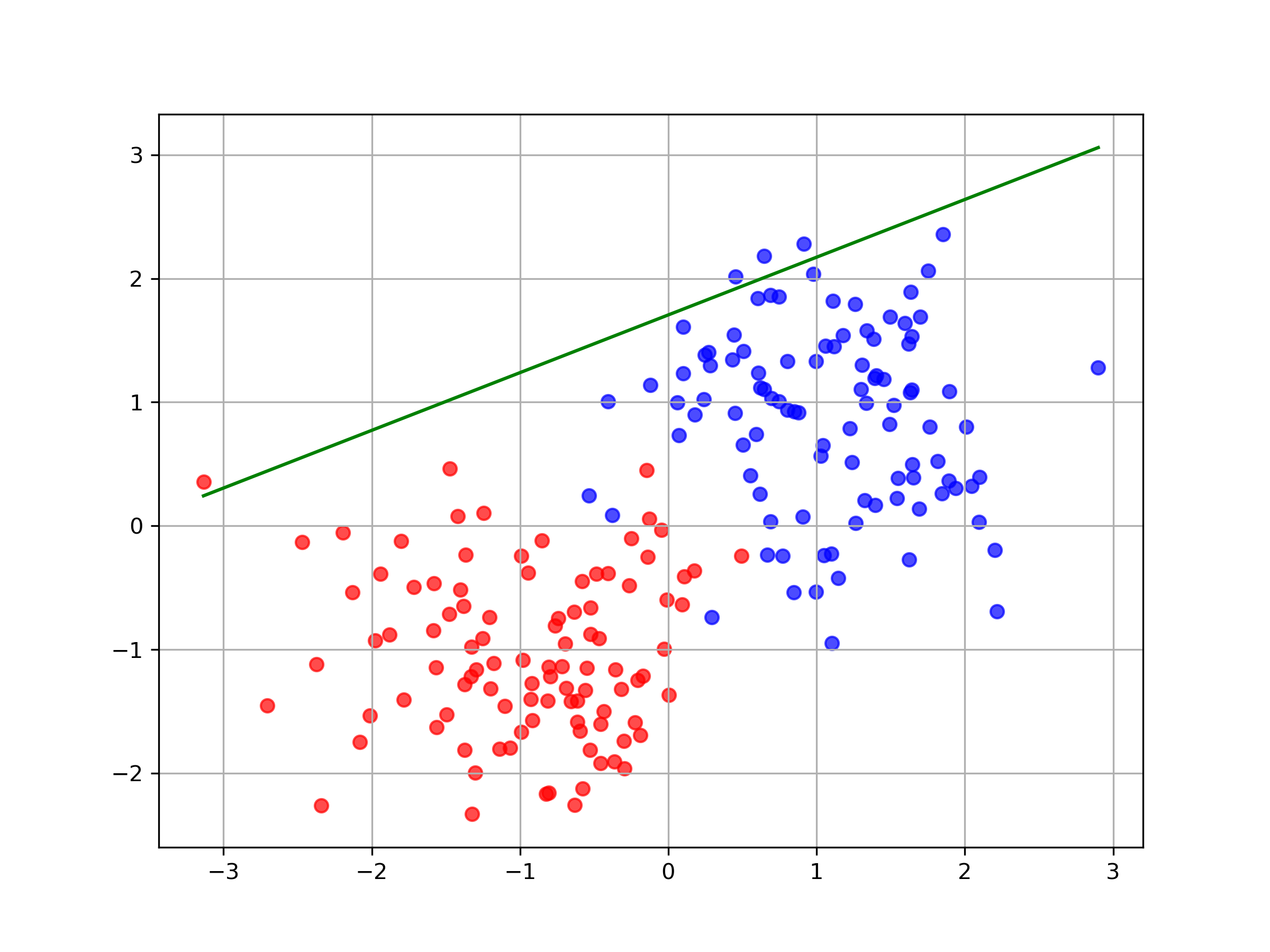
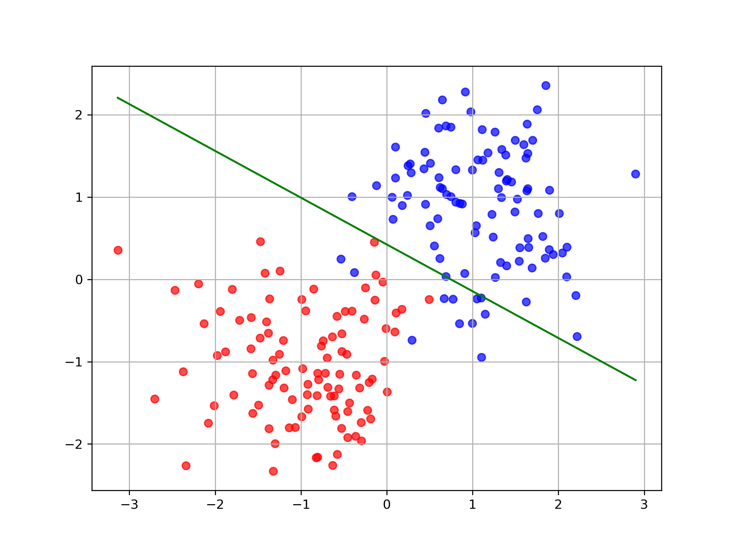
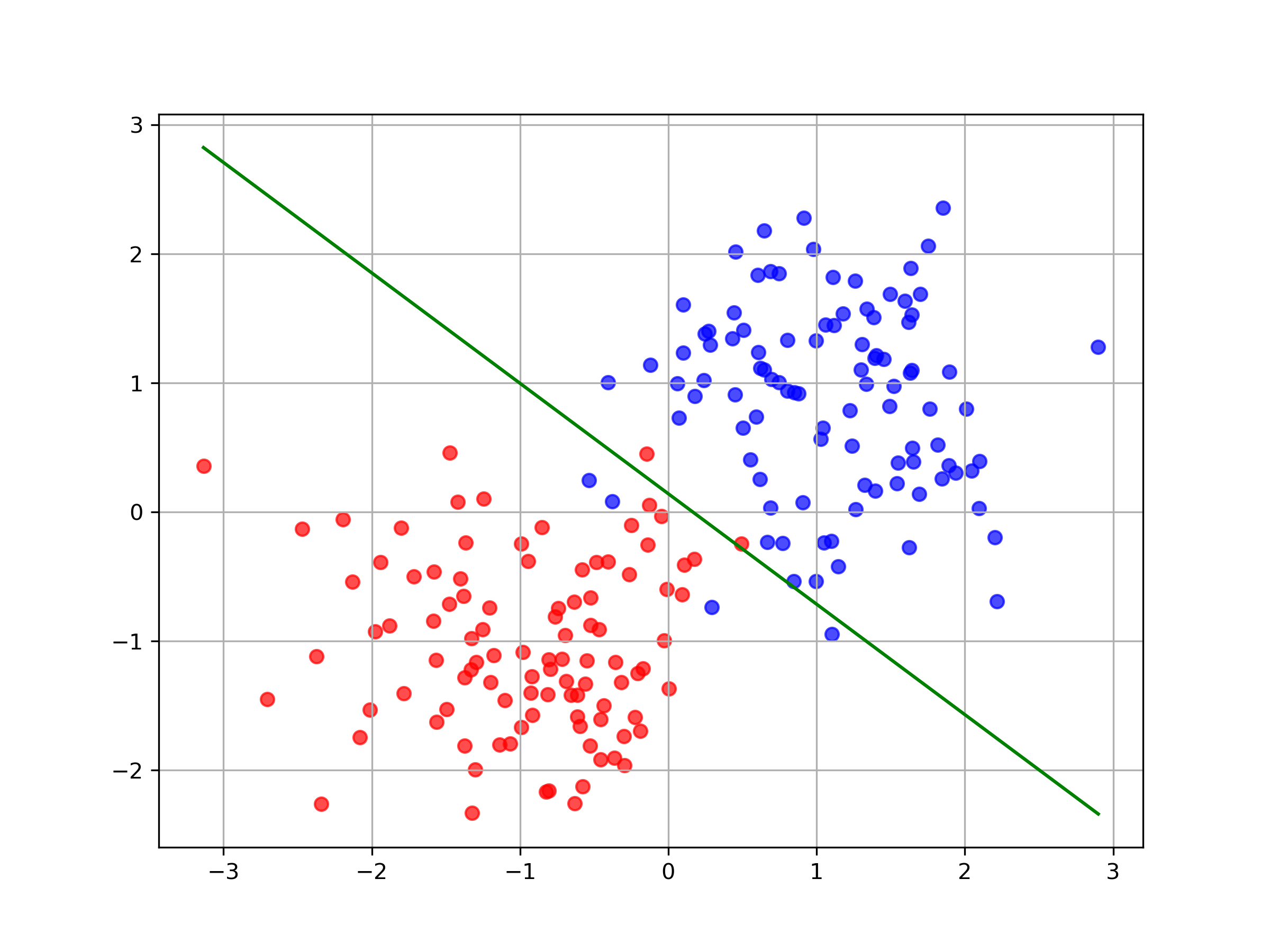
As expected, our model performs quite well on this data and quickly finds the optimal decision boundary. We get around 97% accuracy after couple of hundred training iterations.

A lot of what we covered: maximum likelihood estimation, normalizing raw predictions into probabilities, gradient descent etc. carries over to more complex algorithms. The entire code for the model training and the plotting can be found here.